49
CHAPTER 6: INVENTORY ANALYSIS
6.1 Objective
This chapter is the first on inventory. We use it as an introduction to “supply chain management”
6.2 Additional Suggested Readings
We assign a short case as supplemental reading for the economies of scale. The case is used to show
1. What factors should be taken into consideration when deciding the batch size of a particular type of
printer shipped to Europe (or any other destination)? What do you think of the fact that “inventory
2. Assume that each printer costs HP $100 and the fixed cost incurred in each production run (lost
production due to setup) is $1,000. Consider the Option A printers for world wide demand. How
many of these printers should Vancouver produce in each batch?
Problem 6.1
The data in the question is: flow rate R = 50,000 parts/yr, fixed ordering cost S = $800, purchasing cost C
Problem 6.2
BIM Computers: Assume 8 working hours per day.
Chapter 6
• We know Q = 4 wks supply = 1,600 units; R = 400 units/wk = 20,000 units/yr; purchase cost
•
30.91setups/yr × $2,093.75/setup = $64,718/yr.
Problem 6.3
Victor's data: flow unit = one dress, flow rate R = 30 units/wk, purchase cost C = $150/unit, order lead
time L = 2 weeks, fixed order cost S = $225, cost of capital r = 20%/yr. Victor currently orders ten weeks
supply at a time, hence Q = 10wks × 30 units/wk = 300 units.
a. Costs for Victor's current inventory management:
• Annual variable ordering (purchasing) cost = RC = $150/unit × 30 units/wk × 52 wks/yr
= $234,000/yr.
• Annual fixed ordering (setups) cost = (# of orders/yr) S = (R/Q) S = (30×52/yr/300) $225
= $1,170/yr.
• Annual holding cost = H (Q/2) = (rC) (Q/2) = $30/yr × 150 = $4,500/yr.
• Total annual costs = $239,670.
b. To minimize costs, Victor should order in batches of
Chapter 6
= 50. We must find the fixed cost S2 at which Q2 is optimal. Since Q1 is optimal for S1, we have
Q1 = 400 =
H
R
H
RS 100022 1
=
. So, R/H = 160000/2000 = 80.
Problem 6.5
Major Airlines: This question illustrates the basic tradeoff between fixed and variable costs in a service
industry; thus the concepts of EOQ discussed in class in the context of inventory management are much
more generic.
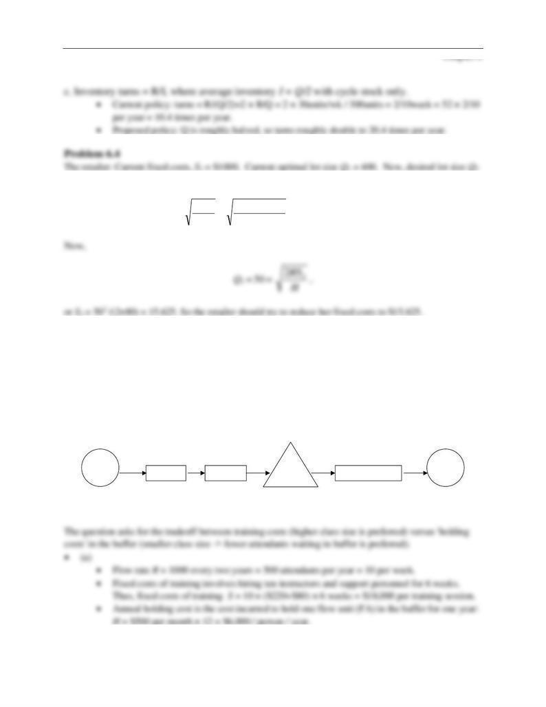
The process view here is illuminating and it goes as follows: flow unit = one flight attendant (FA). The
process transforms an input (= "un-trained" FA) into an output (= "quitted" FA). The sequence of
activities is: undergo training for 6 weeks, go on vacation for one week, wait in a buffer of "trained, but
not assigned FA" until being assigned, serve as a FA on flights, and finally quit the job.
Untrained
FA Training Vacation Pool of
trained FAs Serve on flights Quitted
FA
T = 6 wks 1 wks ? wks 2 years
R
Chapter 6
5.56
t (weeks)
0
I (on vacation)
6 7
55
t (weeks)
0
I (in buffer)
6 7
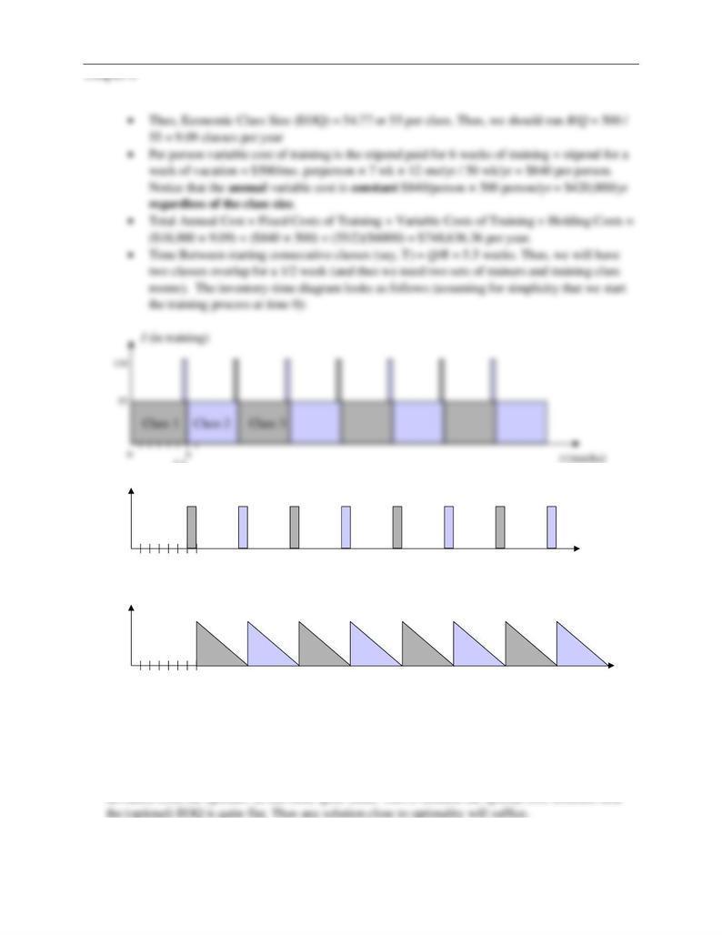
55
Class 1 Class 2 Class 3
Class 1 Class 2 Class 3
• (b): This part of the question illustrates the following: Often, in reality, people wish to adopt policies
that are simple (e.g., starting training every 6 weeks is simpler than trying to track the exact days to
start training when subsequent trainings start every 5.5 weeks. But what is the implication of
deviation from the optimal? In this case, quite small. This is because the optimal cost structure near
Chapter 6
Problem 6.6
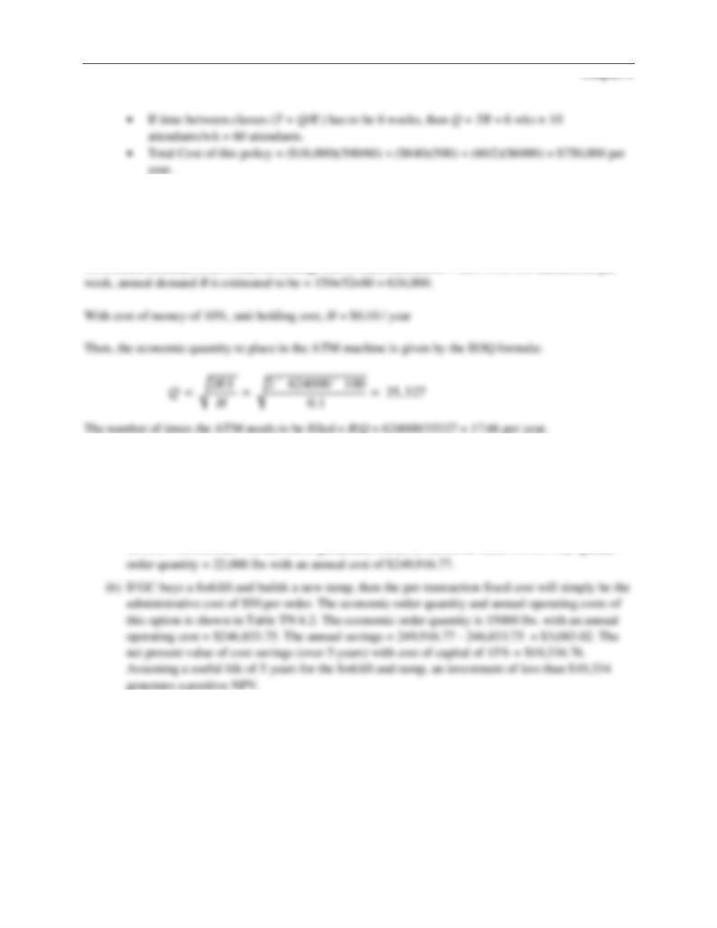
Fixed cost of filling an ATM m/c, S = $100.
To estimate demand, observe that the average size of each transaction = $80. With 150 transactions per
Problem 6.7
The annual demand, R = 150,000 lbs/yr. The purchase price per lb is $1.50. However the shipping cost
exhibits a quantity discount model. The holding cost per year is then 15% of the sum of the purchase and
shipping cost. The administrative costs of placing an order = $50/order.
(a) In addition, rental cost of the forklift truck adds to the fixed cost giving a total fixed cost, S =
50+350 = $400/order. We can use a spreadsheet model as shown in Table TN 6.1. The optimal
Problem 6.8
Changeover time = 4hrs resulting in a fixed cost, S = 4 × 250 = $1,000.
Annual demand, R = 1000/mo × 12 = 12,000 units / yr.
Unit cost, C = 100
Holding cost = $25 / unit / yr.
a) The optimal production batch size is
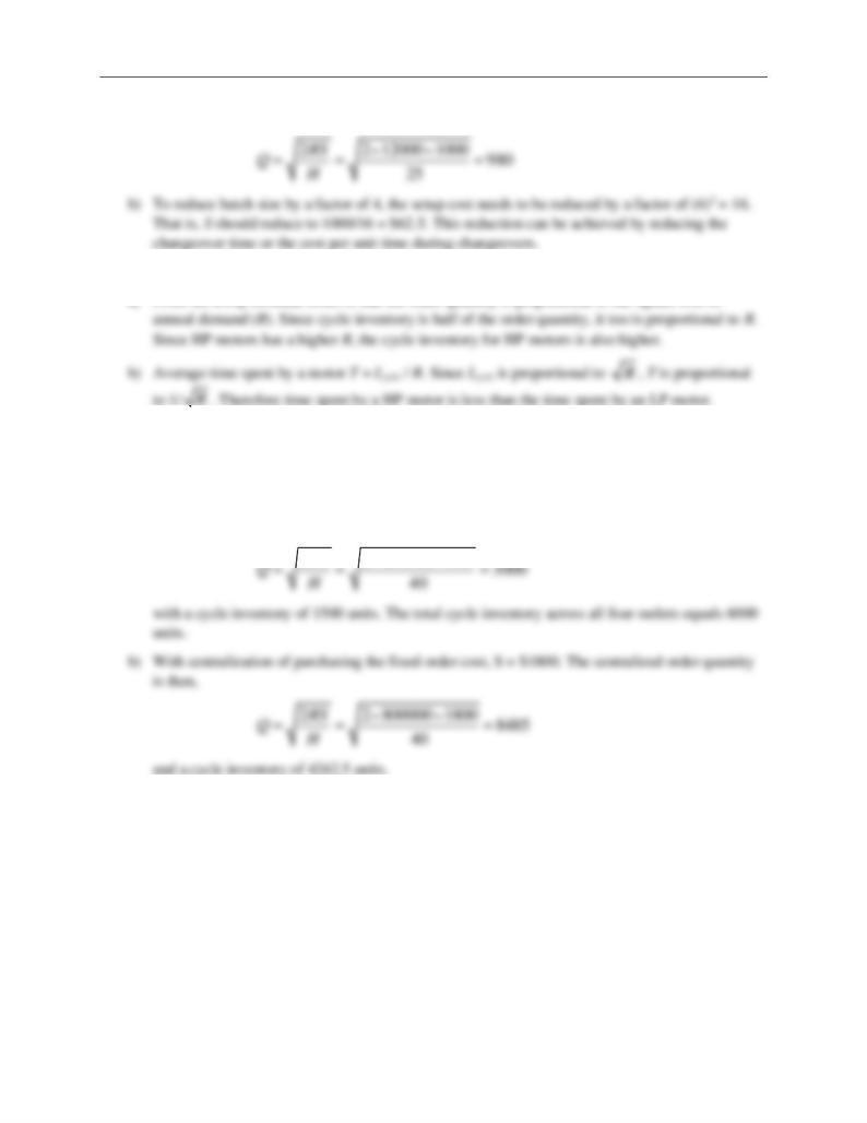
Chapter 6
Problem 6.9
a) From the EOQ formula, observe that the order quantity is proportional to the square root of
R
Problem 6.10
Each retail outlet faces an annual demand, R = 4000/wk × 50 = 200,000 per year. The unit cost of the
item, C = $200 / unit. The fixed order cost, S = $900. The unit holding cost per year, H = 20 % × 200 =
$40 / unit / year.
a) The optimal order quantity for each outlet
2 2 200000 900 3000
RS