
Chapter 9
The IS Curve
◼ Chapter Outline, Overview, and Teaching Tips
Chapter Outline
Planned Expenditure
The Components of Expenditure
Consumption Expenditure
Planned Investment Spending
Net Exports
Government Purchases and Taxes
Goods Market Equilibrium
Solving for Goods Market Equilibrium
Deriving the IS Curve
Understanding the IS Curve
What the IS Curve Tells Us: Intuition
What the IS Curve Tells Us: Numerical Example
Why the Economy Heads Toward Equilibrium
Why the IS Curve Has Its Name and Its Relationship with the Saving-Investment Diagram
Factors That Shift the IS Curve
Changes in Government Purchases
Application: The Vietnam War Buildup, 1964–1969
Changes in Taxes
Changes in Autonomous Spending
Policy and Practice: The Fiscal Stimulus Package of 2009
Changes in Financial Frictions
Summary of Factors That Shift the IS Curve
Chapter Overview and Teaching Tips
90 Mishkin • Macroeconomics: Policy and Practice, Second Edition
1. Planned expenditure is the sum of four types of spending to purchase goods and services:
consumption, planned investment, government, and net exports (exports minus imports). Keynes
2. The consumption function states that consumer spending depends on disposable income, the real interest
rate, and other variables such as consumers’ optimism and wealth. The consumption function is written
as C =
C
+ mpc (Y – T) – cr. Y – T represents disposable income, and mpc is the marginal propensity
3. Planned investment spending consists of fixed investment, which is expenditures by business firms
on equipment and structures and by households on residential housing, and inventory investment,
Chapter 9 The IS Curve 91
4. Firms plan to invest in equipment, structures, and inventories when they expect to earn more from
these forms of physical capital than the interest cost of the funds used for their purchase. When the
real interest rate is very low, the cost of funds is very low, and many of the firm’s planned
6. Net exports are inversely related to the real interest rate. When the real interest rate increases, ceteris
paribus, the expected return on domestic assets rises relative to foreign assets. People’s increased
7. Equilibrium in the goods market requires that total planned spending on goods and services equals
8. If unplanned inventory investment is positive, there is an excess supply of goods because aggregate
output exceeds planned expenditures. When this occurs, firms will cut production, and aggregate
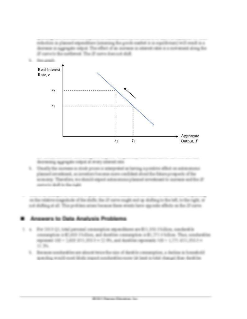
9. The IS curve shows the different combinations of the real interest rate and aggregate output for which
the goods market is in equilibrium with Y = C + I + G + NX. Because consumption, planned
investment, and net exports all are inversely related to the real interest rate, planned expenditures rise
10. The IS curve shifts when autonomous factors (factors that operate independently of the real interest
rate and aggregate output) cause changes in planned expenditures. When an autonomous factor
92 Mishkin • Macroeconomics: Policy and Practice, Second Edition
increases planned expenditures at each real interest rate, the IS curve shifts to the right because the
1. Replacing the given estimates in Equation 1 yields: 16,420 = 12,210 + 1,680 + 2,970 + NX. Solving
2. In order to use Equation 2 to calculate consumption expenditure, we need an estimate of the marginal
2013.
b. Dell’s inventory spending is the change in the level of its inventory during the course of 2014.
On December 31, 2014, Dell’s inventory equals 25,000 $450 = $11,250,000. Therefore, Dell’s
inventory spending in 2014 is $1,250,000 = $11,250,000 – $10,000,000.
5. a. A decrease in U.S. imports of Chinese goods will result in an increase in U.S. Net Exports
(assuming exports do not change), a component of planned expenditure. Assuming the goods
market is in equilibrium, this will increase aggregate output at every interest rate, thereby shifting
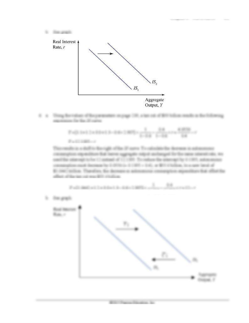
Chapter 9 The IS Curve 93
=−
12.1395
−−
1 0.6 1 0.6
94 Mishkin • Macroeconomics: Policy and Practice, Second Edition
7. a. An increase in interest rates will decrease consumption expenditure, decrease planned investment
spending, and decrease net exports, as summarized by the terms c, d, and x in Equation 10. This
8. a. A more expensive dollar will result in fewer U.S. exports and more U.S. imports (everything else
the same), therefore decreasing Net Exports. Graphically, this shifts the IS curve to the left,
9. This is an example in which it is quite difficult to measure the net effect of these events. Depending
2. a. For 2013:Q1, personal income minus disposable personal income = $13,601.3 billion –
$11,992.2 billion = $1,609.1 billion. This difference represents the amount of taxes households
pay.
Chapter 9 The IS Curve 95
b. For 2012:Q2 to 2013:Q1, personal consumption averaged $11,205.4 billion, and from 2011:Q2 to
2012:Q1 it averaged $10,839.3 billion. Disposable personal income over the same periods
3. a. From 2012:Q2 to 2013:Q1, the average change in investment was $18.75 (billion).
b. From 2012:Q1 to 2012:Q4, the average change in ri was –0.48.
c. The ratio of the changes is 18.75/–0.48 = –39.06; the absolute value of this represents the
coefficient d on the investment function; that is, for every 1 percentage point increase in ri, real
private domestic investment falls by about $39 billion.
d. From 2008:Q3 to 2009:Q2, the average change in investment was –$155.83 (billion), and from
2008:Q2 to 2009:Q1, the average change in ri was 0.86. The coefficient on investment, d during
that period is the absolute value of –155.83/0.86, or d = 181.2. Thus, for every 1 percentage point
increase in ri, real private domestic investment would fall by about $181.2 billion. This is
significantly higher than during the current period; the financial frictions component partly helps
explain the significant decline in investments during the financial crisis period despite real
interest rates being relatively low; however, other factors are clearly at play that pushed the drop
in investment (and hence the increase in the coefficient) much higher than it is today that can’t be
captured by the financial frictions data series (for instance, prospects for long-term growth). In
other words, in order to have the coefficient be comparable to what it is today, the financial
frictions measure would have to be much higher to capture the drop in investment seen during the
financial crisis.
96 Mishkin • Macroeconomics: Policy and Practice, Second Edition
◼ Data Sources, Related Articles, and Discussion Questions
A. For Information About Application: The Vietnam War Buildup, 1964–1969
Data Source
Federal Reserve Bank of St. Louis: http://research.stlouisfed.org/fred2/series/GCEC96?cid=107. Click on
“Edit Graph” and change the years to see the evolution of defense expenditure between 1960 and 1970.
Related Article
Feldstein, Martin, “Rethinking the Role of Fiscal Policy”:
http://www.nber.org/feldstein/RethinkingtheRole.pdf. This article puts in perspective the increase in
government expenditure during the 1960s (Section 1) and discusses the effectiveness of stimulus packages
in general.
Discussion Question
During the period described in the application, unemployment and interest rates were at relatively low
levels for some time, while output increased. Would this mean that an increase in government spending is
the answer to reach low unemployment and economic growth at the same time?

Chapter 9 The IS Curve 97