
Chapter 3
Aggregate Production and Productivity
◼ Chapter Outline, Overview, and Teaching Tips
Chapter Outline
Determinants of Aggregate Production
Factors of Production
Production Function
Cobb-Douglas Production Function
Application: Why Are Some Countries Rich and Others Poor?
Cobb-Douglas Production Function Characteristics
Changes in the Production Function: Supply Shocks
Determination of Factor Prices
Demand for Capital and Labor
Supply of Capital and Labor
Factor Market Equilibrium
Distribution of National Income
Application: Explaining Real Wage Growth
Application: Oil Shocks, Real Wages, and the Stock Market
Concluding Remarks
Chapter Overview and Teaching Tips
This chapter develops one of the basic building blocks for all the macroeconomic analysis throughout this
book, the aggregate production function. Not only is the aggregate production function used in the study of
economic growth, where it plays a central role, it also is a key element of business cycle analysis because
it determines the level of potential output given the factor inputs.
The chapter starts by discussing the fundamental factors of production and develops the Cobb-Douglas

24 Mishkin • Macroeconomics: Policy and Practice, Second Edition
1. The aggregate production function represents the relationship between the quantities of inputs that go
2. Total factor productivity measures the productivity of all inputs. It is the average output produced by
one unit of capital together with one unit of labor. Labor productivity measures the average output
3. The Cobb-Douglas production function is Y = AK0.3L0.7, where Y = output, A = total factor productivity,
4. The Cobb-Douglas production function exhibits constant returns to scale and diminishing marginal
products for each input. Constant returns to scale means that if all inputs increase by an identical
proportion, output rises by that same proportion. For example, if the amounts of capital and labor
used in production are doubled, output also doubles. Diminishing marginal product implies that if
Chapter 3 Aggregate Production and Productivity 25
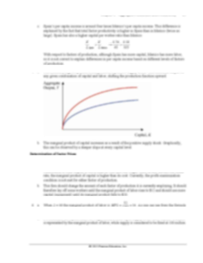
5. Supply shocks are events that either increase or decrease the amount of output that can be produced
with given amounts of capital and labor. In other words, they cause output to change even though
capital and labor have remained the same because they change the productivity of the inputs (the A
6. Factor prices are the prices firms pay for each unit of labor and capital they hire. They pay the wage
rate for each unit of labor they hire and the rental price of capital for each unit of capital they hire.
The explanation of how these factor prices are determined assumes that all firms operate under
7. The profit function is
= P F(K,L) − RK − WL.
denotes economic profits, which are revenues
8. Firms will hire additional units of capital and labor inputs as long as the additional revenue they can
earn by doing so—the marginal product of capital or labor times the average price level—is greater
9. A factor demand curve for capital or labor shows how much of the factor firms will demand at various
real factor prices—the real rental price of capital or the real wage rate of labor—when all other variables
(including amounts of the other factor) are held constant. The negative slopes of the demand curves for
capital and labor result from the production function’s characteristic of diminishing marginal products
and firms’ profit-maximizing decisions to additional units of an input until its marginal product equals
its real factor price. When the real factor price of an input decreases, firms will hire additional units of
26 Mishkin • Macroeconomics: Policy and Practice, Second Edition
10. Equilibrium occurs in a factor market when the quantity of the factor demanded by firms equals the
quantity of the factor its owners offer for sale. The factor price at which this condition is met is the
equilibrium price of the factor. When there is an excess demand, firms want to hire more of the factor
than owners of the factor offer for sale. This occurs when the factor’s price is below the equilibrium
11. Based on the Cobb-Douglas production function and assuming that labor and capital inputs are hired
in perfectly competitive factor markets, national income is divided between labor and capital with the
1. Replacing K and L by 2K and 2L respectively yields:
2. a.
MPL AK L AK
dL dL
−
= = = =
0.74 45
b. Mexico’s per capita income:
1,000,000 $9,524.
105
Y
yL
= = =
Chapter 3 Aggregate Production and Productivity 27
0.74 0.18.
4. a. The unusually high crop yield is interpreted as a positive supply shock. This increases output for
5. a. This firm is not maximizing its profit because it is hiring too many employees and using less
equipment (capital) than it should. At this current real wage, the marginal product of labor (worker’s
contribution to total output) is lower than its cost (the real wage). Also, at this current real rental
0.3
80
for the marginal product of labor, MPL decreases as L increases.
b. To determine the equilibrium real wage, demand must equal supply in the labor market. Demand
28 Mishkin • Macroeconomics: Policy and Practice, Second Edition
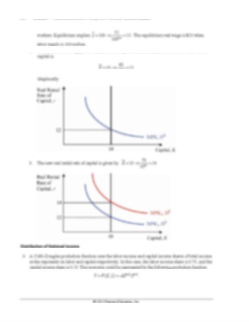
7. a. The intersection of supply and demand in the capital market indicates that the real rental rate of
0.7
10
Chapter 3 Aggregate Production and Productivity 29
9. Your boss is not correct because an important characteristic of a Cobb-Douglass production function
1. a. From 1980 to 2012, nominal wage growth has averaged 4.3 percent, and CPI inflation has
averaged 3.6 percent per year. Thus, inflation has eroded away a substantial part of the
purchasing power of the nominal increase in wages.
2. a. From 2000:Q1 through 2013:Q1, output per person has grown by 28.4 percent; from January
2000 to March 2013, the labor force participation rate fell from 67.3 percent to 63.3 percent, a
decline of 4 percentage points.
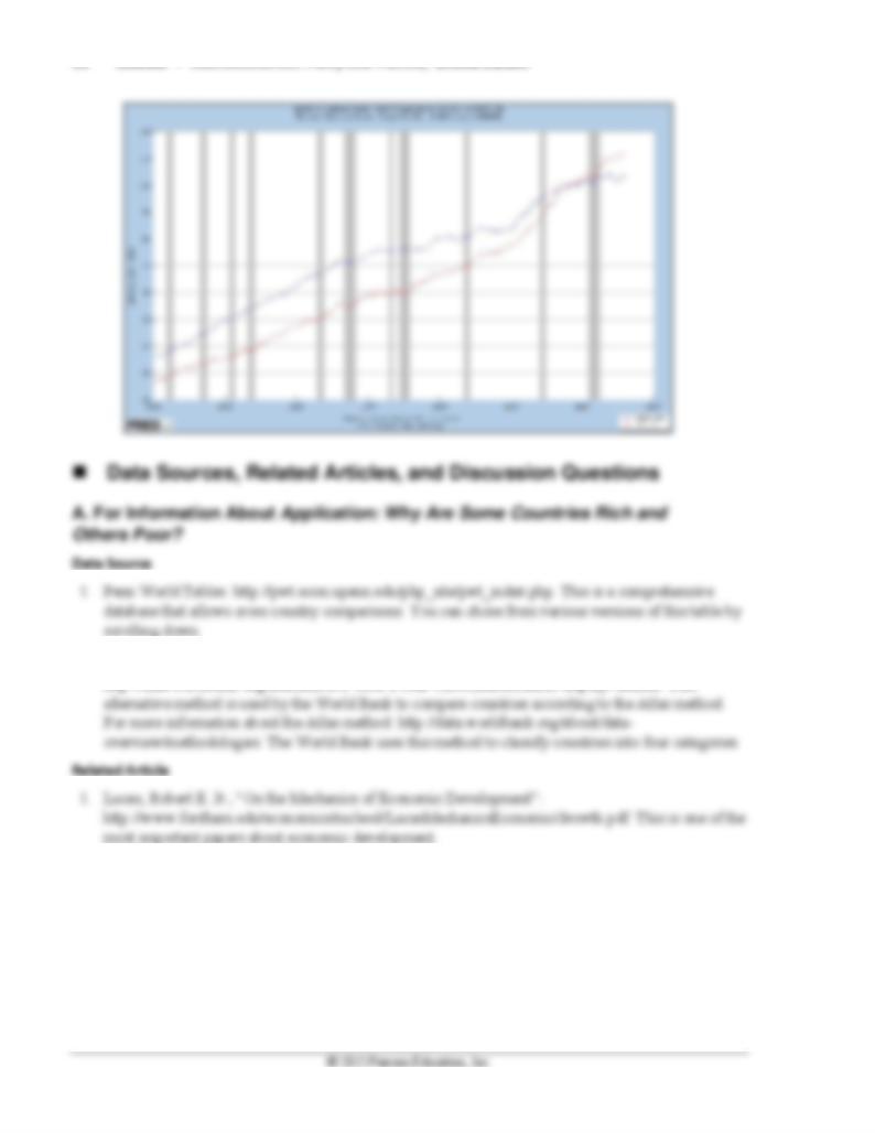
3. a. Generally, labor productivity rises during expansions and declines or does not grow much during
recessions, particularly near the beginning and middle of recessions. Generally, real
compensation per hour rises during expansions and declines or grows slowly during recessions.
b. If output per worker and the MPL are closely linked, then declines in output per worker (MPL)
that happen during recessions should reduce labor demand, and hence the equilibrium real wage,
and vice versa. The labor productivity and real compensation measures seem to support this basic
30 Mishkin • Macroeconomics: Policy and Practice, Second Edition
2. World Bank Classification (Atlas method):
http://data.worldbank.org/indicator/NY.GNP.PCAP.CD/countries/latest?display=default. This
2. Romer, Paul M., “Economic Growth”: http://www.econlib.org/library/Enc/EconomicGrowth.html.
This article discusses various economic growth determinants.
Chapter 3 Aggregate Production and Productivity 31
Discussion Question
The “total factor productivity” term is usually conceived to be a “black box”: it could represent different
technologies, production processes, or even the efficiency of the financial system. Propose different ways
to fill that “black box”: factors that can increase a country’s income per worker (everything else given).
Table 3.2: Select “nonfarm business” for sector, then “real hourly compensation” (real wages) and “Labor
productivity (output per hour)” for measures, and finally “percentage change from same quarter a year
ago” for duration. When done, click “get data.”
Related Article
Greenspan, Alan, “The Revolution in Information Technology”:
http://www.federalreserve.gov/boarddocs/speeches/2000/20000306.htm. In this speech, Greenspan points
out the implications of the revolution in information technology for the U.S. economy.
Discussion Questions
Why do you think that increases in total factor productivity are important for a country as a whole? What
about for an individual in particular?

32 Mishkin • Macroeconomics: Policy and Practice, Second Edition