
Chapter 18
Consumption and Saving
◼ Chapter Outline, Overview, and Teaching Tips
Chapter Outline
The Relationship Between Consumption and Saving
Intertemporal Choice and Consumption
The Intertemporal Budget Constraint
The Intertemporal Budget Constraint in Terms of Present Discounted Value
Preferences
Optimization
The Intertemporal Choice Model in Practice: Income and Wealth
Response of Consumption to Income
Response of Consumption to Wealth
Consumption Smoothing
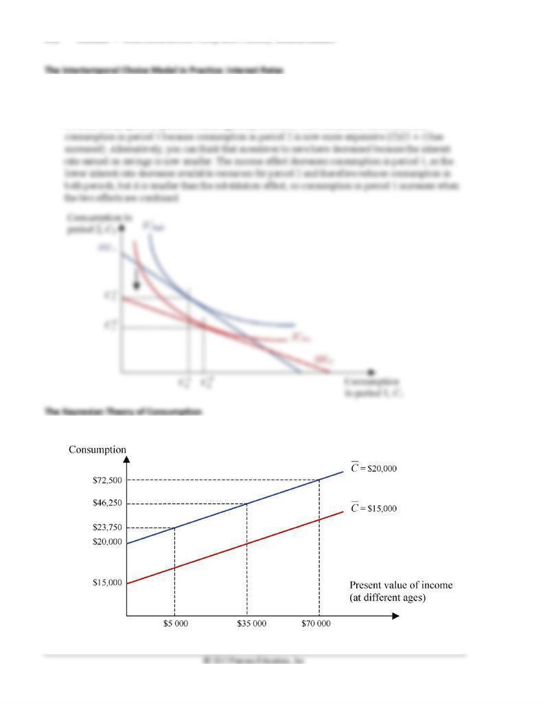
The Intertemporal Choice Model in Practice: Interest Rates
Interest Rates and the Intertemporal Budget Line
The Optimal Level of Consumption and the Intertemporal Budget Line
Borrowing Constraints
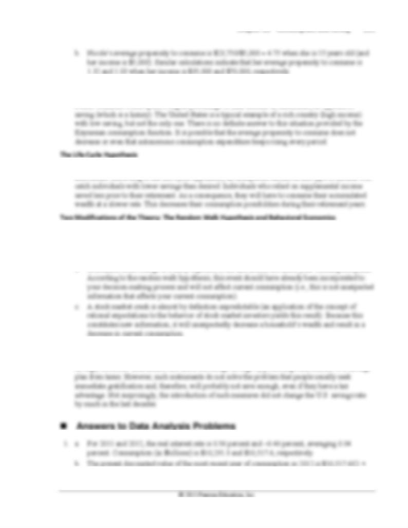
The Keynesian Theory of Consumption
The Keynesian Consumption Function: Building Blocks
Keynesian Consumption Function
The Relationship of the Keynesian Consumption Function to Intertemporal Choice
The Permanent Income Hypothesis
The Permanent Income Consumption Function
Application: Consumer Confidence and the Business Cycle
Relationship of the Permanent Income Hypothesis and Intertemporal Choice
Macroeconomics in the News: The Consumer Confidence and Consumer Sentiment Indices
Policy and Practice: The 2008 Tax Rebate
The Life-Cycle Hypothesis
Life-Cycle Consumption Function
Saving and Wealth Over the Life Cycle

206 Mishkin • Macroeconomics: Policy and Practice, Second Edition
Application: Housing, the Stock Market, and the Collapse of Consumption in 2008 and 2009
Two Modifications of the Theory: The Random Walk Hypothesis and Behavioral Economics
The Random Walk Hypothesis
Behavioral Economics and Consumption
Policy and Practice: Behavioral Policies to Increase Saving
Chapter 18 Web Appendix: Income and Substitution Effects: A Graphical Analysis
Chapter Overview and Teaching Tips
Chapter 18 Consumption and Saving 207
1. Letting S represent private saving, C consumption expenditure, and Y disposable income, it is true
2. The intertemporal budget constraint is based on the idea that a person’s lifetime consumption depends
on (is constrained by) his or her lifetime resources. Borrowing allows people to increase their current
consumption at the expense of future consumption, and saving rewards them for foregoing current
consumption by making possible greater future consumption. The diagrammatic form of the
intertemporal budget constraint rests on several assumptions made by Irving Fisher: There are only
3. Indifference curves show various combinations of current (period 1) and future (period 2)
consumption among which consumers are indifferent (that is, they have no preference for any one
combination over the others) because the combinations all provide the same level of satisfaction (or
happiness or utility). Indifference curves slope downward because consumers will be indifferent
4. The consumer wishes to choose the combination of current and future consumption that will yield the
highest level of satisfaction possible. The intertemporal budget constraint mandates that a consumer’s
current and future consumption lie on the intertemporal budget line. Given this constraint, the highest

208 Mishkin • Macroeconomics: Policy and Practice, Second Edition
5. Increases in current income, future income, and wealth all shift the intertemporal budget line (IBL) to
the right. As a result, current and future consumption both increase. This outcome reflects consumers’
6. Increases in the real interest rate make the IBL pivot around the “no borrowing or lending point” at
which current consumption equals current income plus wealth. If the real interest rate rises, the IBL
becomes steeper (pivots clockwise) to reflect the higher opportunity cost of current consumption and
the higher maximum future consumption that results from higher interest earnings possible on period
1 saving. The impact this has on current and future consumption can be broken into two parts, the
7. Consumers face a binding borrowing constraint if they prefer to consume more than their income in
period 1 but are unable to borrow to do so. This prevents them from achieving the optimal balance
between their current and future consumption. The IBL for these consumers is kinked and becomes a
8. Keynes’s consumption theory is based on the notions that as disposable income rises, consumer
spending also rises, but by a smaller amount, and that consumers spend a smaller proportion and save
a larger proportion of their income as income rises. Keynes assumed that the marginal propensity to
9. Milton Friedman’s permanent income hypothesis divides income into two components, permanent
income that a consumer expects to persist over time (and therefore reflects his or her lifetime
resources) and transitory income that fluctuates over time. The permanent income hypothesis
Chapter 18 Consumption and Saving 209
10. The life-cycle hypothesis assumes that people smooth their consumption over their entire lifetime,
saving some of their income during their working lives to finance their consumption during
retirement. Their lifetime resources consist of earned income and wealth that accumulates as people
11. The random walk hypothesis posits that consumers are forward looking and base their consumption
decisions on their current expectations about future income and lifetime resources. Changes in
consumers’ expectations are unpredictable in that they occur when unanticipated new information
becomes available, so changes in consumption are unpredictable and follow a random walk. In
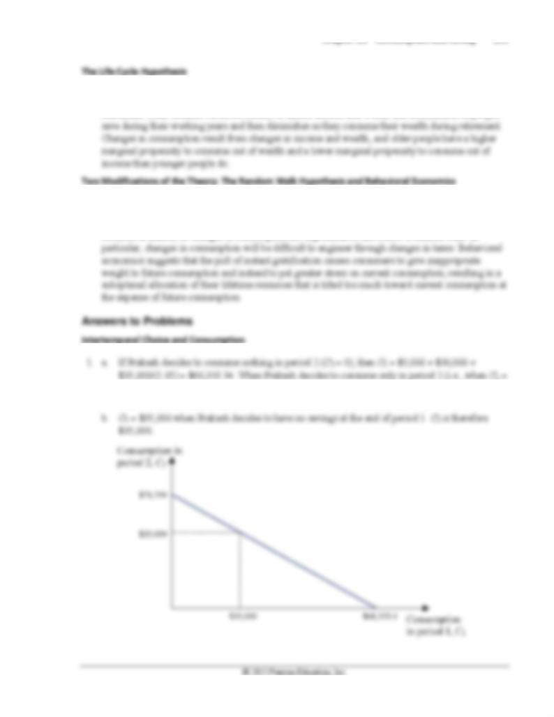
0), then C2 = (1.05) ($5,000 + $30,000 – 0) + $35,000 = $71,750. Thus the intertemporal budget
line intersects the horizontal axis at C1 = $68,333.34 and the vertical axis at C2 = $71,750.
210 Mishkin • Macroeconomics: Policy and Practice, Second Edition
2. a.
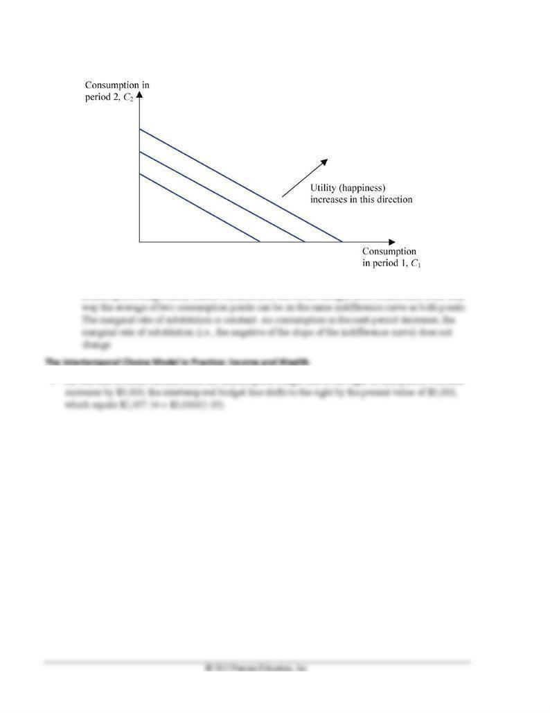
b. Maria’s indifference curves are straight lines (note that these are indifference curves, not
intertemporal budget lines). Maria’s indifference curves are straight lines because this is the only
3. An increase in future income shifts the intertemporal budget line to the right. If next period’s income
Chapter 18 Consumption and Saving 211
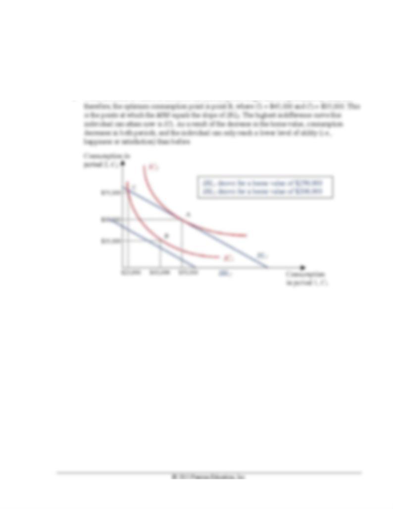
4. a. When the home is valued at $250,000 the intertemporal budget line is represented by IBL1, and
therefore, the optimum consumption point is point A, at which C1 = $55,000 and C2 = $50,000.
This is the point at which the MRS equals the slope of IBL1. The highest indifference curve this
individual can attain is IC2. Although point C is on the same IBL1, it is not the optimum, as this
individual can reach a higher indifference curve (IC2 instead of IC1).
b. When the home is valued at $200,000 the intertemporal budget line is represented by IBL2, and
212 Mishkin • Macroeconomics: Policy and Practice, Second Edition
5. A decrease in the interest rate rotates the intertemporal budget line counterclockwise. The new
intertemporal budget line shares the point at which the individual has no savings at the end of period
1 (i.e., when the individual consumes exactly the value of his or her wealth and period 1 income). As
a result, consumption in period 2 unambiguously decreases. The substitution effect increases
6. a.
Chapter 18 Consumption and Saving 213
7. According to the Keynesian consumption function, a rich country should have a lower average
propensity to consume than a poorer country does because the rich country has a higher income.
Poorer countries would spend a higher percentage of their income on necessities, as opposed to
8. Pensions and other types of supplemental income during retirement play a significant role for many
individuals. According to the life-cycle hypothesis, an unexpected decline in this type of income will
9. a. If taxes increase by less than expected, individuals’ disposable income will be higher than
expected, which will result in higher current consumption. According to the random walk
hypothesis, current consumption will increase, even if taxes have increased because individuals
were already expecting a decrease in their disposable income.
b. Graduation from college is a fairly expected event and should not affect your consumption plans.
10. The application of behavioral economics ideas to consumption behavior concludes that measures like
the creation of IRAs would not have a significant effect on individuals’ consumption (and therefore
savings) decisions. Instruments like IRAs encourage savings by protecting contributions to a savings
0.0004) = $10,513.4.
214 Mishkin • Macroeconomics: Policy and Practice, Second Edition
about 2.9 percent between the two four quarter periods. However, the average of the APC was
essentially constant (increased ever so slightly). The behavior of the APS seems to reinforce this, as
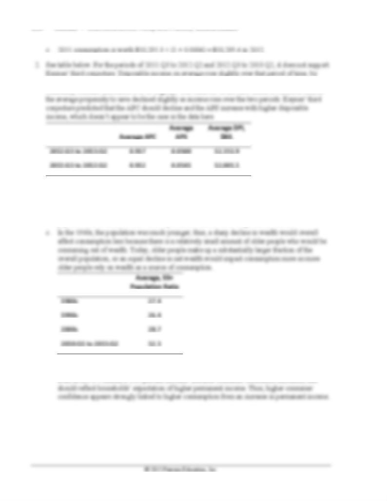
3. a. See table below.
b. The population went slightly “younger” from the 1980s to the 1990s, suggesting under the life-
cycle hypothesis that the MPC out of permanent income should increase over that time. In the
1990s onward, those 55 years and older became an increasingly larger fraction of the whole
population, as a result, the MPC out of permanent income on average should decrease.
4. Yes, they behave as expected. From 2011:Q4 to 2012:Q4, the consumer sentiment index
increased by 79.4 – 64.8 = 14.6. Over the same time, consumption grew to $10,584.8 billion,
from $10,373.1 billion, a 2.04 percent increase. Because consumer confidence increased, this
Chapter 18 Consumption and Saving 215
1. The substitution effect refers to how an individual’s consumption in periods 1 and 2 would respond to
a change in the relative price of consumption in each time period, holding his or her wealth and
income in each period constant. This relative price is given by the slope of the intertemporal budget
2. The income effect is an individual’s response to a change in his or her income when the relative price
3. According to the substitution effect, because the higher real interest rate increases the reward for
saving in period 1, Carmencita will save more in period 1, reducing her consumption in period 1 and
increasing her consumption in period 2. According to the income effect, the higher real interest rate
216 Mishkin • Macroeconomics: Policy and Practice, Second Edition
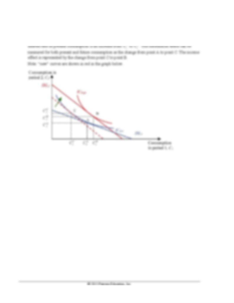
4. As shown in the graph, an increase in the interest rates shifts the intertemporal budget clockwise,
from IBL1 to IBL2 (this shifts is represented by the green arrow). In this case, the income effect is
assumed to be larger than the substitution effect, and therefore, the consequence of an increase in the
B
Chapter 18 Consumption and Saving 217
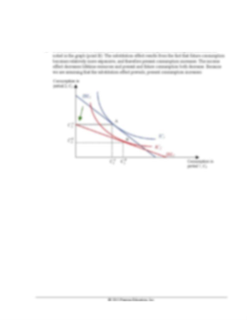
5. a. When the interest rate decreases, the intertemporal budget line pivots counterclockwise, from
IBL1 to IBL2. Note that both IBL lines share one point (the point at which the individual saves
nothing after period 1).
b. If the income effect is smaller than the substitution effect, present consumption increases, as

218 Mishkin • Macroeconomics: Policy and Practice, Second Edition
6. a. The change in the intertemporal budget line from IBL1 to IBL2 is the result of a decrease in the
interest rate, as the intertemporal budget line has a slope equal to: – (1 + r).
b. The substitution effect on present consumption derived from the decrease in the interest rate is
$150 (calculated as the difference between $500 and $650). The decrease in the interest rate
makes future consumption relatively more expensive, and the individual increases his or her
present consumption. This is obtained by applying the new slope of the intertemporal budget line
to the original indifference curve IC1 (represented as point B in the graph). There is also an
income effect, as the decrease in the interest rate decreases the value of lifetime resources.
According to the graph, the income effect on present consumption is the change from $650 to
$700 (or $50). Present consumption increases by $200, and the larger effect is the substitution
effect.
◼ Data Sources, Related Articles, and Discussion Questions
A. For Information About Application: Consumer Confidence and the Business
Cycle
Data Source
Federal Reserve Bank of St. Louis database (FRED):
http://research.stlouisfed.org/fred2/series/UMCSENT. Here you can find data about the University of
Michigan consumer sentiment index.
Related Article
Bloomberg, “Consumer Confidence in U.S. Plunges to Lowest Since 2009 on Jobs Outlook”:
http://www.bloomberg.com/news/2011-08-30/u-s-consumer-confidence-drops-to-lowest-since-09-
as-index-slumps-to-44-5.html. This article details the drop in consumer sentiment that occurred in
fall 2011.

Chapter 18 Consumption and Saving 219
Discussion Question
Determine the effect on consumer confidence, and therefore on autonomous consumption, of news
that indicates a deterioration of economic conditions in the future.
220 Mishkin • Macroeconomics: Policy and Practice, Second Edition

Chapter 18 Consumption and Saving 221