
Chapter 13
Macroeconomic Policy and Aggregate
Demand and Supply Analysis
◼ Chapter Outline, Overview, and Teaching Tips
Chapter Outline
The Objectives of Macroeconomic Policy
Stabilizing Economic Activity
Stabilizing Inflation: Price Stability
Establishing Hierarchical Versus Dual Mandates
The Relationship Between Stabilizing Inflation and Stabilizing Economic Activity
Monetary Policy and the Equilibrium Real Interest Rate
Policy and Practice: The Federal Reserve’s Use of the Equilibrium Real Interest Rate, r*
Response to an Aggregate Demand Shock
Response to a Permanent Supply Shock
Response to a Temporary Supply Shock
The Bottom Line: The Relationship Between Stabilizing Inflation and Stabilizing Economic Activity
How Actively Should Policy Makers Try to Stabilize Economic Activity?
Lags and Policy Implementation
Policy and Practice: The Activist/Nonactivist Debate Over the Obama Fiscal Stimulus Package
The Taylor Rule
The Taylor Rule Equation
The Taylor Rule Versus the Monetary Policy Curve
The Taylor Rule in Practice
Policy and Practice: The Fed’s Use of the Taylor Rule
Inflation: Always and Everywhere a Monetary Phenomenon
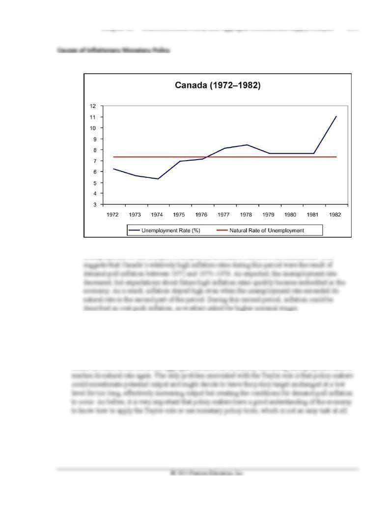
Causes of Inflationary Monetary Policy
High Employment Targets and Inflation
Application: The Great Inflation
Monetary Policy at the Zero Lower Bound
Deriving the Aggregate Demand Curve with the Zero Lower Bound
The Disappearance of the Self-Correcting Mechanism at the Zero Lower Bound
Chapter 13 Macroeconomic Policy and Aggregate Demand and Supply Analysis 137
Application: Nonconventional Monetary Policy and Quantitative Easing
Liquidity Provision
Asset Purchases
Quantitative Easing Versus Credit Easing
Management of Expectations
Policy and Practice: Abenomics and the Shift in Japanese Monetary Policy in 2013
Chapter Overview and Teaching Tips
Chapter 13 shifts the perspective by bringing a new set of actors into the AD/AS framework: policy
makers. We look at how they react to shocks to the economy in order to stabilize both inflation and economic
activity. One unique feature of the dynamic AD/AS framework in this book is that it can address policy
138 Mishkin • Macroeconomics: Policy and Practice, Second Edition
1. Stabilizing economic activity and price stability are the two primary objectives of macroeconomic
stabilization policy. Stabilizing economic activity requires keeping unemployment at the natural rate
2. Policy makers should not strive to achieve zero rates of unemployment and inflation. Even at full
employment, unemployment is not zero because of the existence of frictional and structural
unemployment. Frictional unemployment is beneficial to the economy as it arises from the search
3. A hierarchical mandate gives top priority to the objective of price stability. Under this mandate,
policy makers may pursue the goal of stabilizing economic activity only if it does not compromise
4. The equilibrium real interest rate is the real interest rate that keeps the quantity of aggregate output
5. Stabilization policy is conducted more frequently using monetary policy rather than fiscal policy
Chapter 13 Macroeconomic Policy and Aggregate Demand and Supply Analysis 139
6. The divine coincidence exists when policies that are appropriate to achieve price stability also
stabilize economic activity. When it prevails, policy makers have easier jobs because there is no
tradeoff between policy objectives and they do not have to choose between them. They can, in other
words, have their cake and eat it, too. The divine coincidence prevails when the economy is beset
with aggregate demand shocks or permanent supply shocks but not when it experiences temporary
supply shocks. When faced with either of the first two shocks, policy makers can stabilize both
inflation and economic activity by enacting policies to shift the economy’s aggregate demand curve
and return to long-run equilibrium at potential output. In the case of a temporary supply shock,
however, policies that shift the aggregate demand curve to achieve price stability will move the
economy further away from potential output and those aimed at stabilizing economic activity at
potential output will cause the inflation rate to change.
How Actively Should Policy Makers Try to Stabilize Economic Activity?
7. Activists see the process of price and wage adjustments that move the economy to long-run
equilibrium as working very slowly. They argue that instead of waiting for these slow adjustments to
move the economy to full employment and potential output, government policy makers instead
8. Activists argue that wages are inflexible and, in particular, that they are not likely to fall as would be
needed for the self-correcting mechanism to adjust to long-run equilibrium if the economy suffers
9. The data lag is the time it takes to collect and process the quarterly, monthly, and other data that tell
policy makers how well or poorly the economy is performing. The recognition lag is the time
policymakers may wait for additional data to come in to be more confident of their interpretations of
economic conditions and trends. The legislative lag is the time it takes to decide on a particular
policy. This generally is not long for monetary policy makers but can be quite long for fiscal policy
10. The Taylor rule advises the Fed to raise the real federal funds rate target when the inflation gap or the
output gap rises, and to lower this target rate when those gaps shrink. Inasmuch as it recommends
raising the real interest rate in response to an increase in inflation, it relates directly to the upward
140 Mishkin • Macroeconomics: Policy and Practice, Second Edition
11. There are a number of reasons why this would not be a good idea. There is no guarantee that the
Taylor rule coefficients are stable across time and no one, policy makers included, knows the size of
inflation and output gaps at any given time. Even if policy makers did have accurate information
about the current size of these gaps, relying solely on the Taylor rule would force them to disregard
12. Monetary policy makers can target any inflation rate they want to simply by implementing autonomous
monetary policy easing (to target a higher inflation rate) or tightening (to target a lower one). However,
13. Cost-push and demand-pull inflation result when policy makers in pursuit of high targets for output
and employment (and hence low targets for the unemployment rate) implement policies that raise
aggregate demand when their targets are not met. The two types of inflation both arise from events
that move the economy away from long-run equilibrium, but their initiating causes differ. Cost-push
inflation starts with temporary negative supply shocks or wage increases in excess of productivity
growth. These shift the short-run aggregate supply curve up and to the left and cause output and
employment to fall. Policy makers respond by increasing aggregate demand, which raises output and
employment but also increases inflation. Following this accommodating policy, workers now have an
incentive to push for further excessive wage increases because they have obtained higher wages but
14. When the zero lower bound is hit, a lower inflation rate leads to a higher real interest rate because the
nominal interest rate is fixed at zero, and this higher real interest rate than causes planned expenditure
Chapter 13 Macroeconomic Policy and Aggregate Demand and Supply Analysis 141
15. A negative output gap leads to a fall in the short-run aggregate supply curve, which lowers inflation,
16. All unconventional policies work by lowering the interest rate for investments and so stimulate
investment spending and shift the aggregate demand curve to the right. Liquidity provision helps to
heal impaired financial markets, thereby lowering financial frictions and, hence, the real interest rate
for investments. Asset purchases of private securities raise the price of these securities, thereby
1. a. According to Section 8 of the Reserve Bank of New Zealand Act of 1989, the Central Bank of
New Zealand has a clear hierarchical mandate to achieve low and stable inflation. The idea
behind such a mandate is that stabilizing prices will create the proper conditions for economic
2. a. According to aggregate demand and supply analysis, the decrease in government expenditures
results in a shift to the left in the aggregate demand curve, as aggregate expenditure decreases at
every inflation rate. As a result, the new intersection point with the short-run aggregate supply
curve determines a lower inflation rate and output level than before. At this point, output is below
3. According to aggregate supply and demand analysis, a less efficient economy will end up in a new
long-run equilibrium at a lower level of output. Depending on the monetary policy response, the
inflation rate might be higher than before the implementation of reforms that made the economy less
efficient or might remain unchanged. In any event, output is lower in the long run. This is why the
142 Mishkin • Macroeconomics: Policy and Practice, Second Edition
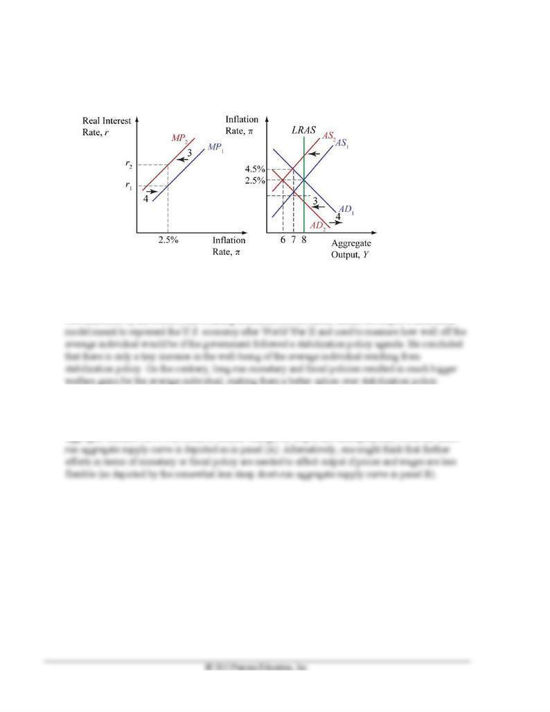
4. a. Changes described by data suggest that policy makers decided to stabilize inflation in the short
run, with the corresponding decrease in output, during period 3.
b. Labeled arrows in the graph refer to the table time periods.
How Actively Should Policy Makers Try to Stabilize Economic Activity?
5. Evidence that shows that the welfare gains from stabilizing output and unemployment are relatively
small, which supports the nonactivist case. This is actually a major topic in macroeconomics, which
was addressed by the Nobel Prize-winning economist Robert Lucas. Lucas developed a theoretical
6. In panel (A) the short-run aggregate supply curve has a steeper slope, meaning that wages and prices
in general are more flexible (i.e., changes in output result in larger changes in the inflation rate). This
situation constitutes a stronger argument in favor of nonactivist policy because changes in the
aggregate demand curve will result in smaller changes in output and unemployment when the short-
Chapter 13 Macroeconomic Policy and Aggregate Demand and Supply Analysis 143
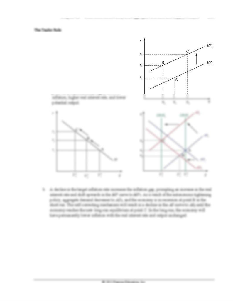
7.
a.
The decline in potential output shifts the LRAS
curve to the left. The lower potential output
increases the output gap, prompting an
autonomous tightening of policy and a shift of
the MP curve to MP2. In the short-run, the
economy ends up at point B. As a result of the
self-correcting mechanism, the AS curve shifts
up, resulting in higher inflation and raising the
real interest rate along MP2. Eventually the
economy reaches the new long-run equilibrium at
point C, at a permanently higher level of
144 Mishkin • Macroeconomics: Policy and Practice, Second Edition
Chapter 13 Macroeconomic Policy and Aggregate Demand and Supply Analysis 145
8. a.
b. According to the graph, Canada’s unemployment rate was below the estimated natural rate of
unemployment for the first part of the period, and then it was above the natural rate. This
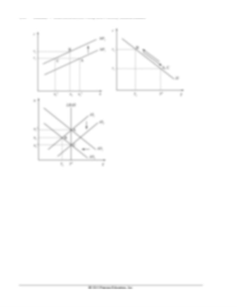
9. The Taylor rule suggests that the policy rate target should be increased when the output gap is
positive. This rule is perfectly consistent with avoiding demand-pull inflation. The natural rate of
unemployment is the unemployment rate at which output is at its potential level. A positive output
gap means that the economy is producing more output, a situation in which unemployment is below
its natural rate. Therefore, increasing interest rates at every inflation rate (shifting the MP curve up)
results in a shift to the left in the aggregate demand curve, thereby increasing unemployment until it
146 Mishkin • Macroeconomics: Policy and Practice, Second Edition
10. a. Policy makers were worried that a shock could push the economy into a deflationary spiral, in
which the short-term nominal policy rate would be bound at the zero lower bound. At that point,
conventional monetary policy would be ineffective. Policy makers viewed the risk of economic
damage in the event of a deflationary spiral to be significant enough to overcome any potential
inflation risk in implementing the policy. Thus, policy makers chose to err on the side of
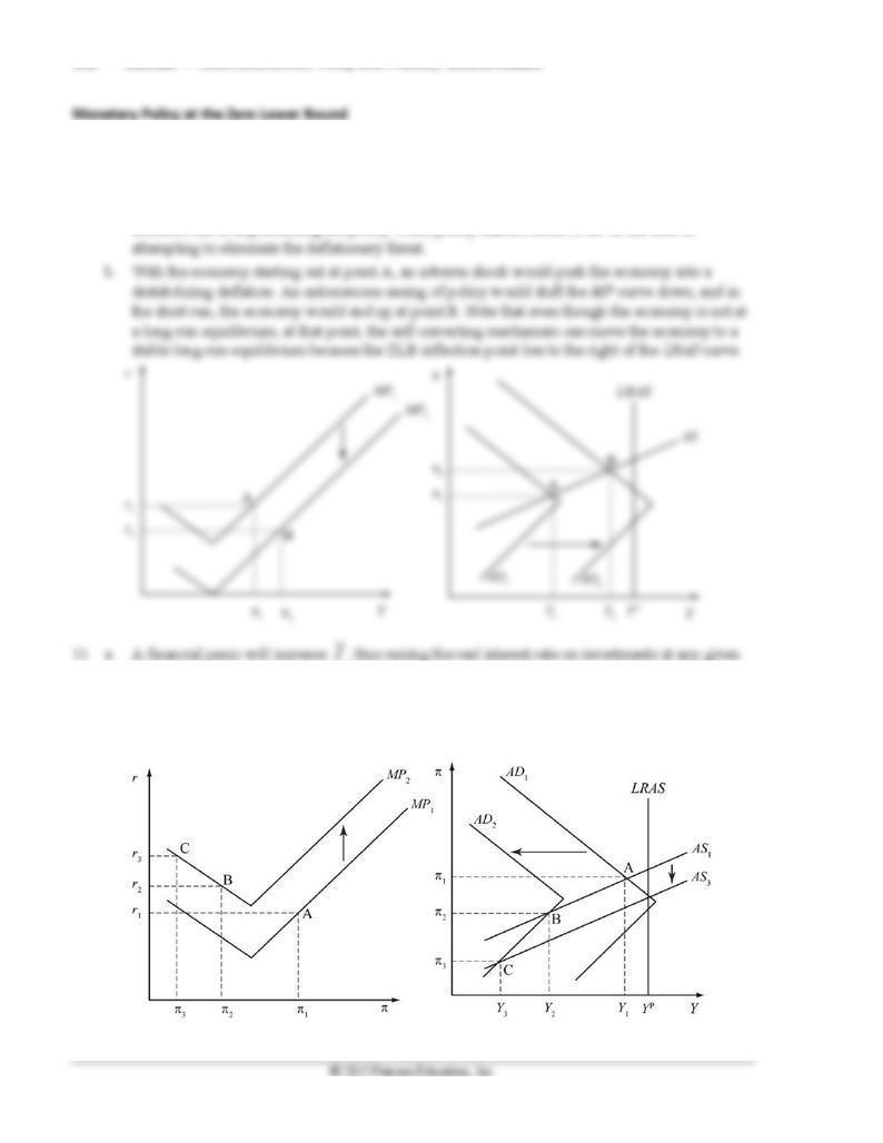
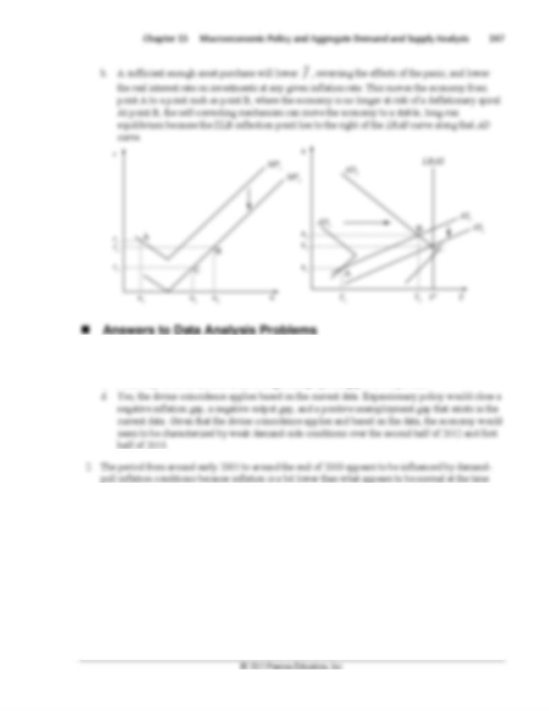
11. a. A financial panic will increase
, thus raising the real interest rate on investments at any given
inflation rate. A sufficiently large panic will push the economy to point B, where the self-
correcting mechanism will lower inflation, and real rates will rise because the economy is beyond
the ZLB. This results in a deflationary spiral in which the economy will move toward (and past) a
point such as point C.
1. a. From 2012:Q2: 2013:Q1, the average inflation gap was –0.5 percent.
b. From 2012:Q2: 2013:Q1, the average output gap was –5.7 percent.
c. From July 2012 to June 2013, the average unemployment gap was 2.2 percent.
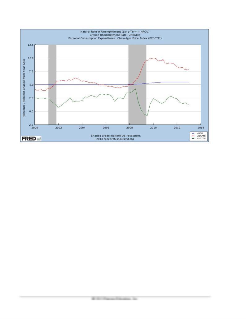
(2.5 percent), and the unemployment rate rises and remains above the estimated natural rate during
this time. For a brief time from the middle of 2007 to the middle of 2008, the economy appears to be
hit by a cost-push inflation episode because the inflation rate spikes and the unemployment rate rises
above the natural rate of unemployment. From the middle of 2008 to the most current period, the
middle of 2013, inflation remains at or below what appears to be the longer term trend of 2.5 percent,
while the unemployment rate is well above the natural rate, suggesting that demand-pull forces are at
work.
148 Mishkin • Macroeconomics: Policy and Practice, Second Edition
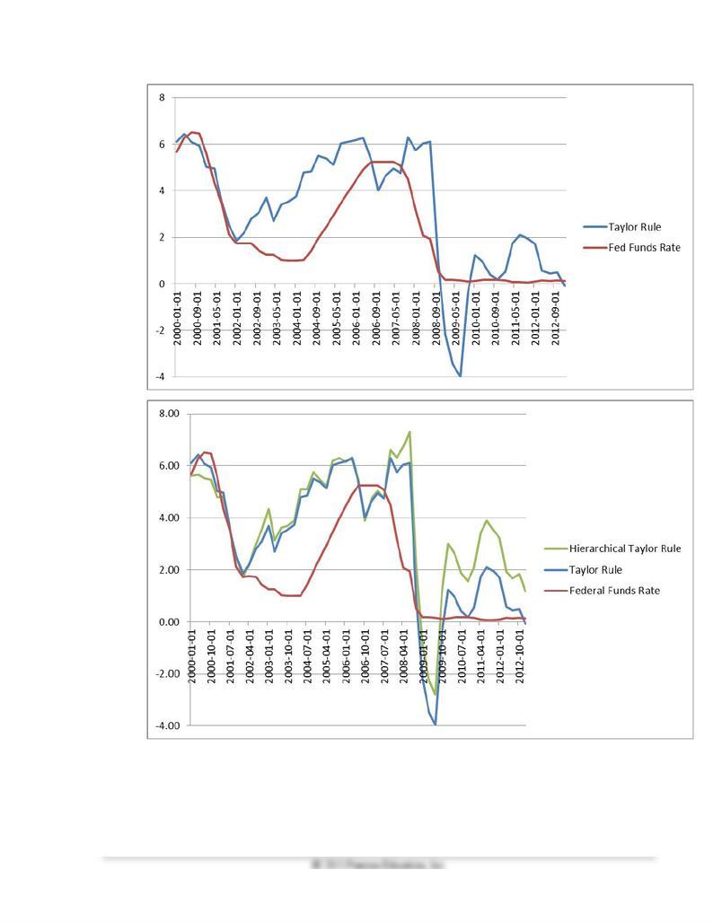
a. For the most recent period in 2013:Q1, the Fed Funds Rate is 0.14 percent, while the Taylor Rule
predicts a slightly negative –0.07 percent, representing a gap of 0.21 percent. Compared to other
significant deviations, this seems to be a fairly close correspondence, although the negative value
is not possible in practice.
b. See graph below. The Taylor rule since 2000 has periods in which they are fairly closely
correlated, particularly from 2000 to 2002. However, there are significant gaps in other times, or
periods in which they do not seem to move together, such as the period from 2002 to 2006. From
2008 onward, there are significant differences between the two, particularly the period late in
2008 through 2010, in which the Taylor rule predicts the Fed Funds Rate should be negative by
as much as almost –4 percent, which is not possible. It also predicted a significant rise in the fed
funds rate in 2011, which did not materialize.
c. Because the Fed funds rate was at the zero lower bound during that time, conventional monetary
policy through adjustments in the fed funds rate was not possible, and highlights a limitation of
the Taylor rule: under “normal” conditions the Taylor rule provides a good approximation to
appropriate fed funds rate policy. However in extreme situations such as the financial crisis
period, the Taylor rule is less useful because other (unconventional) monetary policy tools are
needed to achieve stimulus.
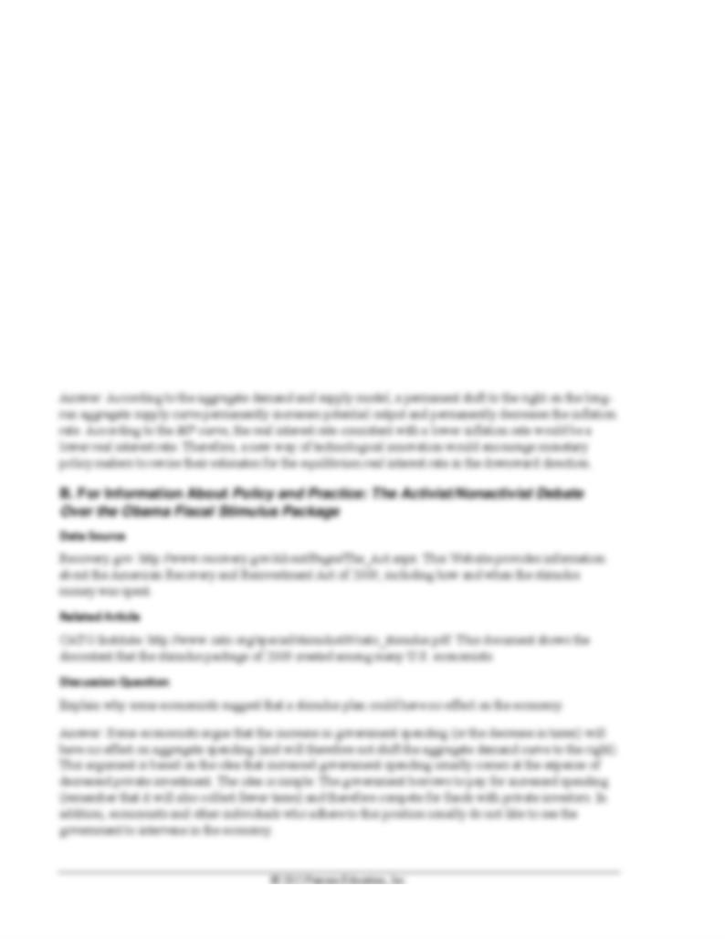
d. See graph below. For the most part, the baseline Taylor rule and the hierarchical Taylor rule
predict nearly the same fed funds paths. The only significant deviations are from 2008 onwards,
where it predicts a significantly higher fed funds rate due to the inflation spike during that time.
Since 2010, it would predict a fed funds rate around 2 percent, which is much higher than during
that time and what the baseline rule predicts. For the current period, under such a hierarchical
Taylor rule, the fed funds rate would be predicted to be about 1.2 percent, much higher than the
current 0.14 percent.
Chapter 13 Macroeconomic Policy and Aggregate Demand and Supply Analysis 149
150 Mishkin • Macroeconomics: Policy and Practice, Second Edition
◼ Data Sources, Related Articles, and Discussion Questions
A. For Information About Policy and Practice: The Federal Reserve’s Use of
the Equilibrium Real Interest Rate, r*
Data Source
Federal Reserve System: http://www.federalreserve.gov/monetarypolicy/fomc_historical.htm. From this
page you can access previous blue and green books. There are also short descriptions of these publications.
Related Article
Federal Reserve System: FOMC Transcripts and Other Historical Materials, 2004.
http://www.federalreserve.gov/monetarypolicy/files/FOMC20040128bluebook20040122.pdf . This is the
January 27–28, 2004 FOMC Meeting bluebook. Note the Policy Alternatives on page 7 of this document
and the subsequent projections made by the FOMC staff.
Discussion Question
Suppose a new wave of technological innovation shifts the long-run aggregate supply curve to the right.
Everything else the same, what would be the effect on the equilibrium level of the real interest rate?
Chapter 13 Macroeconomic Policy and Aggregate Demand and Supply Analysis 151
152 Mishkin • Macroeconomics: Policy and Practice, Second Edition
Chapter 13 Macroeconomic Policy and Aggregate Demand and Supply Analysis 153