CHAPTER 5
A Closed-Economy One-Period
Macroeconomic Model
KEY IDEAS IN THIS CHAPTER
1. A new section has been added on “A Model of Public Goods: How Large Should
4. End-of-chapter problems have been added.
TEACHING GOALS
There are three key points to be learned from this chapter. The first point is that when we
allow the consumers and firms that we studied in Chapter 4 to interact with each other
and with the government, the economy is able to achieve equilibrium through price
adjustment. In this particular case, the “price” is the relative price of leisure, the real
wage. The second important point is that the equilibrium that markets settle upon is a
favourable one, in the sense of Pareto optimality. This point is in keeping with Adam
Smith’s notion that the “invisible hand” of self-interested individuals, meeting in a
competitive market, can work for the common good. The third point is that we can
discover directly the equilibrium position of a market economy by solving an economic
planner problem. Although students may find this point to be somewhat arcane,
emphasize the fact that it will be much simpler to solve problems (e.g., exam problems)
by working with a planner problem as opposed to solving directly general equilibrium
problems.
Once students have mastered the mechanics of the model, the two problems for which
this model is best suited are the analyses of changes in government spending and total
factor productivity. In working on these problems, stress the applicability of these results
to historical applications and as a guide to understanding current events.
The model is then modified, so that some fiscal policy issues can be addressed. This
modification involves including a proportional tax on wage income. This is interesting, as
this gives us a departure from Pareto optimality, and allows us to illustrate a general
principle—the Laffer curve.
In the baseline version of the model in this chapter, government spending simply
represents a resource cost for the economy as a whole, which is fine for analyzing some
types of spending on national defense, for example, or simply for studying the resource
implications of government spending. However, for other purposes, it can be useful to
study the public-goods role of government spending, which is done in the final section in
the chapter. The model is simplified so that the optimal choice of government spending
can be studied. Optimal government spending increases with GDP, and with the
efficiency of government activity.
CLASSROOM DISCUSSION TOPICS
An alternative approach to this material is to start with the example of Robinson Crusoe
(or Castaway, Gilligan’s Island, etc.). Does an isolated individual have any economic
choices? What would guide these choices? Would you rather be on an island with a more

Chapter 5: A Closed-Economy One-Period Macroeconomic Model
plentiful food supply? A pure income effect can then be presented in the form of extra
food (or a volleyball) washing up on shore, or in the form of pirates (government?)
demanding tribute. An increase in total factor productivity can be in the form of obtaining
a fishing net or a ladder to climb coconut trees, etc.
The next step would be to ask students about the likely consequences of having additional
individuals on the island. If they are all identical, and there are no economies to team
production, will there be any reason for markets to exist? Could a market improve things?
How and why? Typically, markets improve things only to the extent that people are
different. However, these types of differences are what we are willing to ignore when we
adopt the fiction of a representative consumer.
An important effect of the increase in total factor productivity, as explained in this
chapter, is that of an increase in the welfare of the representative consumer. One way to
highlight the importance of technological innovation, and hence the increased total factor
productivity, would be to ask students if they currently hold full-time jobs. If so, how
many hours have they worked during the past work week? Compare their work hours
with the number of hours per week a typical worker worked in 1901: a worker in the
Canadian manufacturing sector worked about 55 hours per week.
However, the average work week in the manufacturing sector in Canada shortened
steadily into the 1970s. Real wages in Canada increased sharply during the early
twentieth century. These wage increases were driven by technological innovation and
increased total factor productivity, and therefore were largely permanent. The reduced
work hours per week is an optimal response of a worker in the Canadian manufacturing
sector.
It may also be noted that workers in richer countries with higher wage rates (for example,
the U.S. and Canada) tend to work fewer hours per week than workers in poorer countries
with lower wage rates (for example, the Philippines and Sri Lanka). Because the cross-
country differences in wages reflect long-term differences in factor productivity, the
evidence that workers in high-wage countries have shorter work weeks supports the
finding that permanent increases in the real wage induce workers to supply less labour.
Issues associated with the Laffer curve came up in the United States in the 1980
Presidential election when Ronald Reagan was first elected. This was, of course, long
before the typical intermediate macro student was born, so the instructor will need to do
some work to make this relevant. The incentive issues to do with income taxation are
certainly relevant, and have been driving reductions in marginal income tax rates (at the
top end of the income distribution) in many countries for at least 30 years. A discussion
of marginal tax rates vs. average tax rates would be useful.
The last section in the chapter provides a simple model for determining the optimal size
of the government. This is the starting point for a discussion of the role of government,
and how economists think about the tradeoff between government and private activity.
What gives the government an advantage in some types of activities relative to the private
sector? How large should the government be? How well do we as a society do in
determining the size of our government?

2. Competitive Equilibrium
a) Equilibrium Modelling
i) Endogenous and Exogenous Variables
3. Optimality
a) Pareto Optimality
b) Welfare Theorems
i) First Theorem: A Competitive Equilibrium Can be Pareto Optimal
4. Effects of an Increase in Government Purchases
a) Impact Effect
i) Parallel Downward Shift in PPF
ii) Pure Income Effect
b) Equilibrium Effects
i) Reduced Consumption
Chapter 5: A Closed-Economy One-Period Macroeconomic Model
5. A Change in Total Factor Productivity
a) Impact Effect
i) Upward Shift in PPF
ii) Steeper PPF
(4) Real Wages Rise over Time
6. A Distorting Tax on Wage Income, Tax Rate Changes, and the Laffer Curve
a) A Simplified One-Period Model with Proportional Income Taxation.
7. A Model of Public Goods: How Large Should the Government Be?
a) Basic model
1. Although we often think about the negative externalities of congestion and pollution
in cities, there may also be some positive externalities. A concentrated population is
better able to support the arts, professional sports, etc; cities typically have a greater
variety of good restaurants and so forth. Perhaps a more basic issue is that there may
be some increasing returns to scale at low output levels that make industrial
production more costly in small towns. There may also be externalities in production
2. In a one period model, taxes must be exactly equal to government spending. A
reduction in taxes is therefore equivalent to a reduction in government spending. This
3. A reduction in the capital stock.
a) This works exactly the same as for the increase in total factor productivity in
Figures 5.9 and 5.10, except in reverse, that is, the PPF shifts down. Output falls,
employment may rise or fall (because of offsetting income and substitution
effects), leisure may rise or fall (likewise), consumption falls, and the real wage
falls.
Chapter 5: A Closed-Economy One-Period Macroeconomic Model
4. Government productivity.
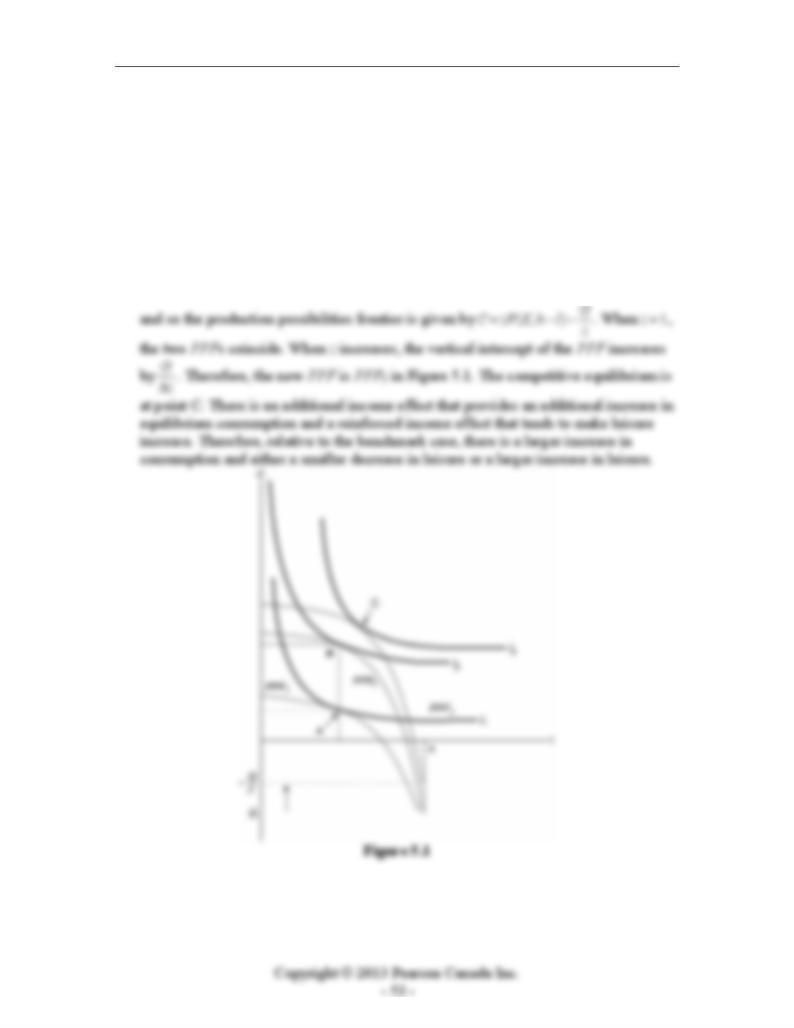
First consider the benchmark case in which 1z=, and there is no effect of changes in z
on government activities. Now suppose that z increases. This case of an increase in z
is depicted in Figure 5.1 below. The original production possibilities frontier is
labelled PPF1 and the competitive equilibrium is at point A. If the increase in z only
affects the economy through the change in ),( NKzF , then the new production
possibilities frontier is PPF2. The diagram shows a case in which the income and
substitution effects on leisure exactly cancel out, and the economy moves to point B.
The equation for the production possibilities frontier is (, )CzFKhl T=−−. In the
benchmark case, TG= and so we have (, )CzFKhl G=−−. For this problem, /TGz=,

Instructor’s Manual for Macroeconomics, Fourth Canadian Edition
5. Change in preferences.
a) At the margin, the consumer decides that leisure is preferred to consumption. That
is, the consumer now requires a bigger increase in consumption to willingly work
more (consume less leisure). In more intuitive language, the consumer is lazier.
b) To work out the effects of this change in tastes, we refer to Figure 5.2. The
production possibility frontier in this example is unchanged. The consumer now
picks a new point at which one of the flatter indifference curves is tangent to the
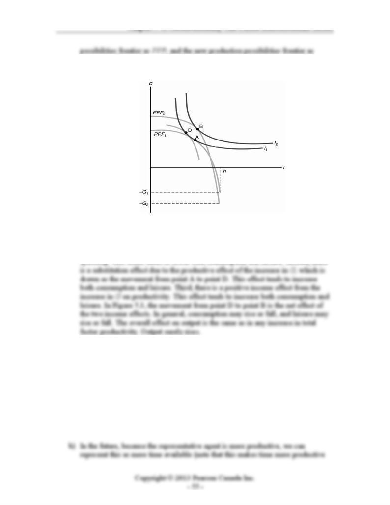
6. Production-enhancing aspects of government spending.
a) The increase in government spending in this example has two separate effects on
the production possibilities frontier. First, the increase in government spending
Chapter 5: A Closed-Economy One-Period Macroeconomic Model
PPF2. If the production-enhancing aspects of the increase in government spending
are large enough, representative consumer utility could rise, as in Figure 5.3.
Figure 5.3
b) There are three effects at work in this example. First, there is a negative income
effect from the increase in taxes needed to pay for the increased government
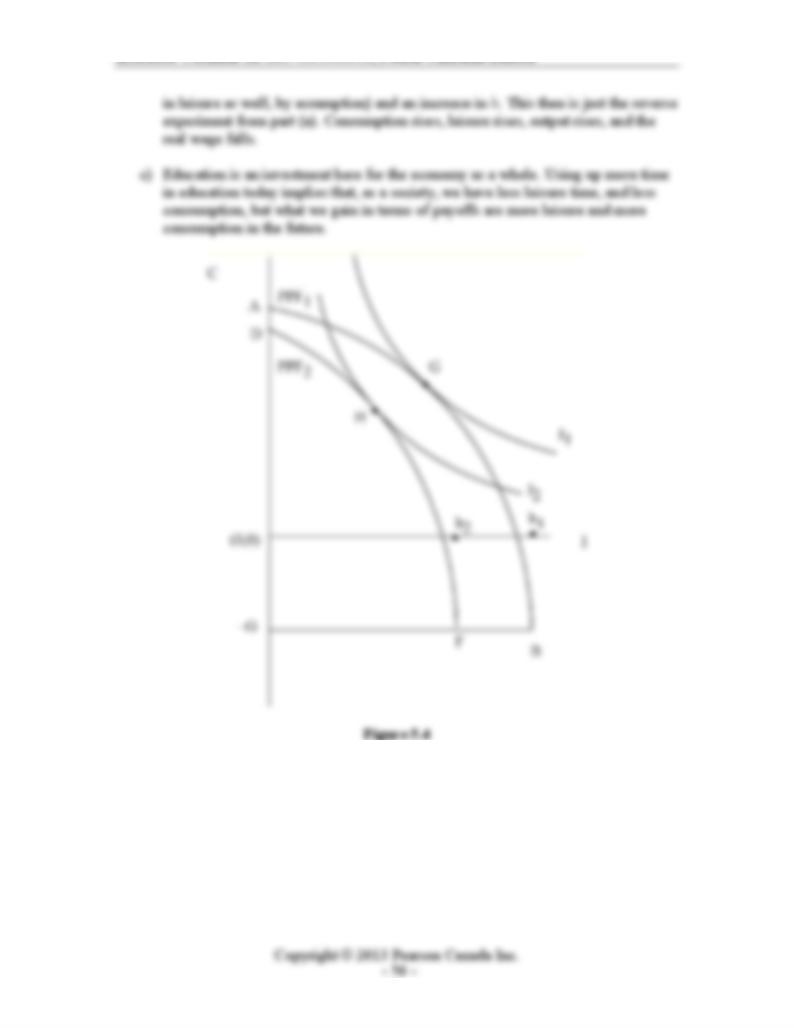
7. Increase in hours spent in education
a) In the present, an increase in the quantity of hours used up for the representative
consumer in education can be represented in the model as a decrease in the
quantity of time available, h, from h1 to h2 in the figure. This shifts the PPF to the
left by a fixed amount h2 – h1 for each quantity of consumption. This will then
have a similar income effect to a reduction in government spending. Consumption
and leisure must fall, but note that the quantity of leisure must fall by less than the
decrease in available hours, so hours worked must fall. Therefore output falls in
the present. The real wage rises, just as for a decrease in G.
Instructor’s Manual for Macroeconomics, Fourth Canadian Edition
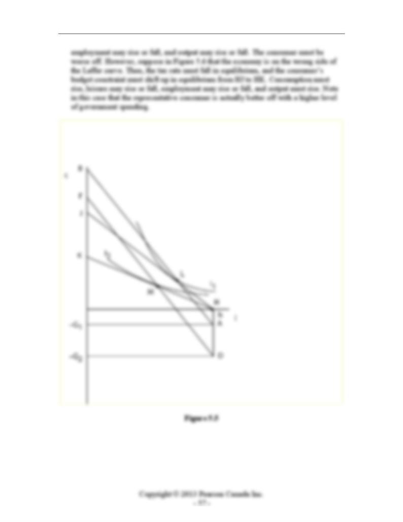
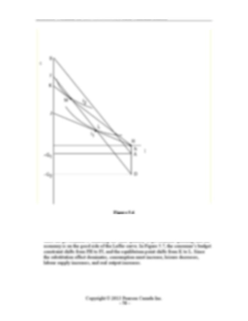
8. Increase in government spending with a proportional wage income tax.
In the Figure 5.5, the production possibilities frontier is initially AB, and it shifts to
DF with an increase in G. If the economy is on the good side of the Laffer curve, then
with the consumer’s budget constraint in equilibrium initially given by HJ, the
consumer must face a higher tax rate in the new equilibrium, facing a budget
constraint like HK. The equilibrium point shifts from L to M. If we disentangle the
income and substitution effects, consumption must fall, leisure may rise or fall,
Chapter 5: A Closed-Economy One-Period Macroeconomic Model
Instructor’s Manual for Macroeconomics, Fourth Canadian Edition
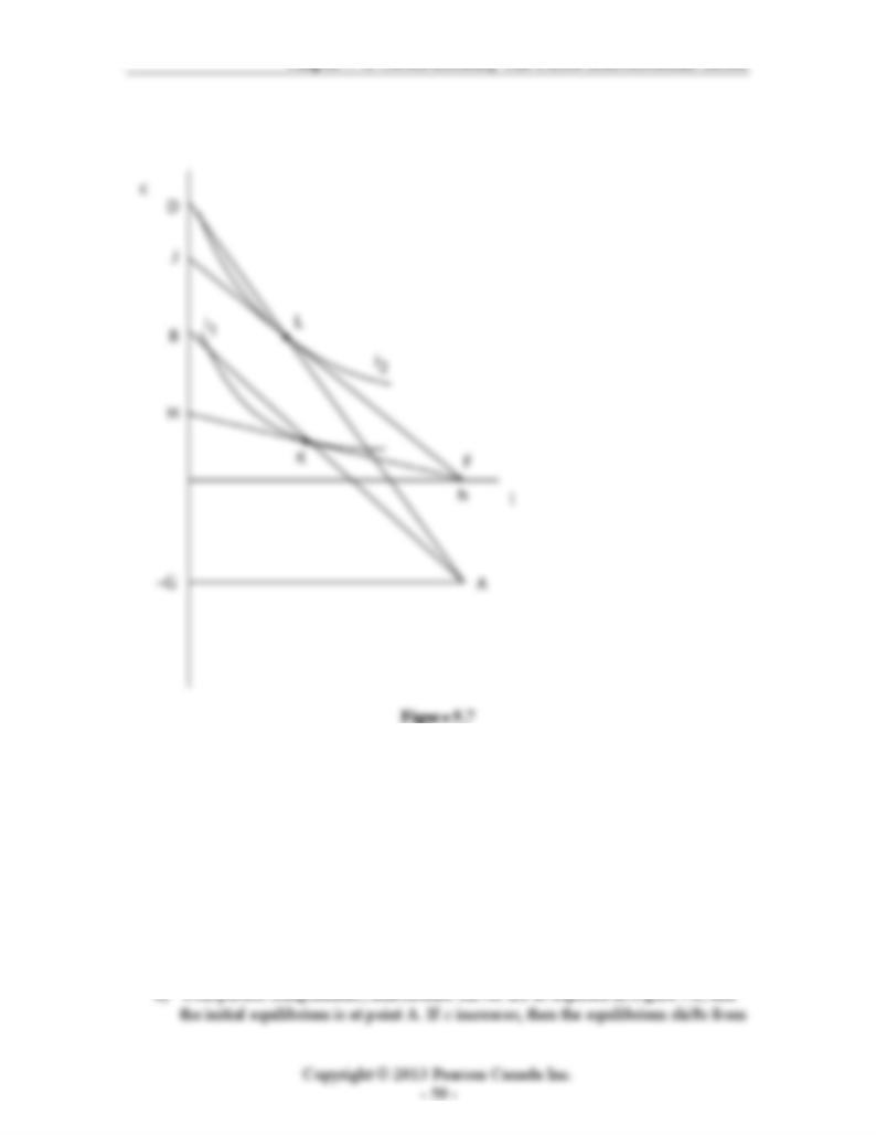
9. In Figure 5.7, the production possibilities frontier shifts to the right from AB to AD.
Since the substitution effect dominates the income effect on labour supply, the Laffer
curve shifts up for each tax rate, and so the tax rate must be lower in equilibrium,
Chapter 5: A Closed-Economy One-Period Macroeconomic Model
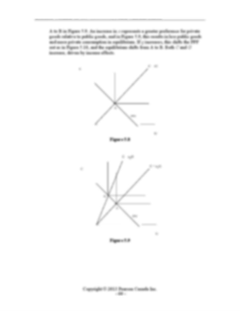
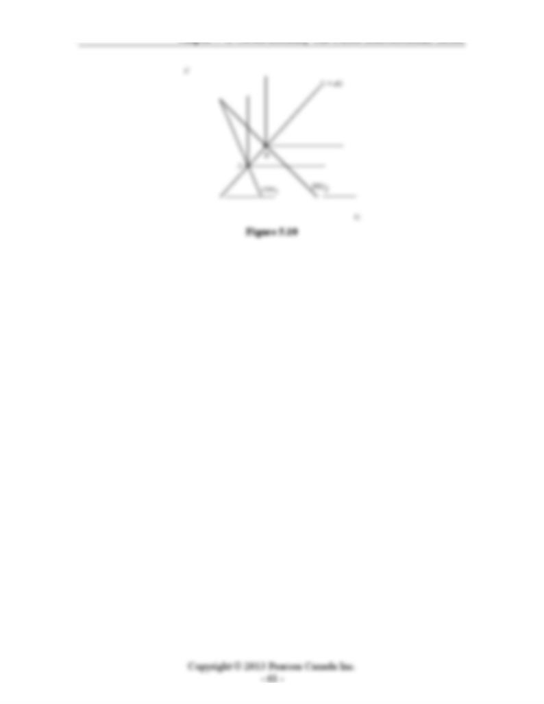
10. a) With perfect substitutes preferences, indifference curves are straight lines with
slope –b, where b is the marginal rate of substitution. If b > 1/q, so that the
indifference curves are steeper than the PPF, then the optimal choice for the
government is G=qY, so that C = 0. Thus if b is relatively large (the consumer
cares relatively more about public goods relative to private goods) and q is
relatively large (the government is relatively efficient), then all production should
be carried on by the government. Alternatively if b < 1/q, then G = 0 and C = Y,
so that government is inactive. Thus, if b increases or q increases, this makes it
more likely that b > 1/q and we have the first case, where all production comes
from the government.
Instructor’s Manual for Macroeconomics, Fourth Canadian Edition
Chapter 5: A Closed-Economy One-Period Macroeconomic Model