Your assignments hero!
You have an assignment questions. We have the answers. Let's get started.
Numerical Methods For Engineers And Scientists: An Introduction With Applications Using Matlab 3 Chapter 4
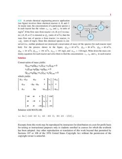
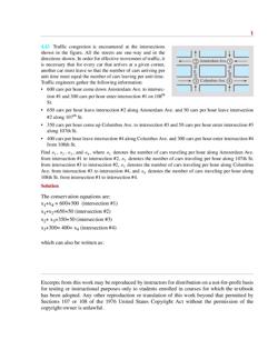
1 Excerpts from this work may be reproduced by instructors for distribution on a not-for-profit basis for testing or instructional purposes only to students enrolled in courses for which the textbook has been adopted. Any other reproduction or translation of this work beyond that permitted by 4.41 A certain chemical engineering process application (see figure) involves three chemical reactors A, B, and C. At steady state, the concentrations of a particular species n in each reactor has the values , , and in units of mg/m3. If the flow rates from reactor i (A, B, or C) to reac- tor j
Numerical Methods For Engineers And Scientists: An Introduction With Applications Using Matlab 3 Chapter 4
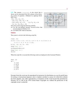
1 Excerpts from this work may be reproduced by instructors for distribution on a not-for-profit basis for testing or instructional purposes only to students enrolled in courses for which the textbook has been adopted. Any other reproduction or translation of this work beyond that permitted by 4.39 The currents, , in the circuit that is shown can be determined from the solution of the follow- ing system of equations. (Obtained by applying Kirch- hoff’s law.) , , Solve the system using the following methods. (a) Use the user-defined function GaussJordan that was developed in Problem 4.22. (b) Use MATLAB’s built-in functions.
Numerical Methods For Engineers And Scientists: An Introduction With Applications Using Matlab 3 Chapter 4
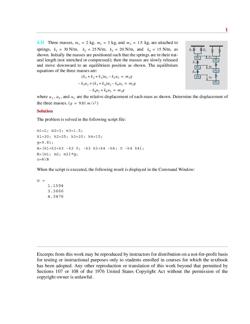
1 Excerpts from this work may be reproduced by instructors for distribution on a not-for-profit basis for testing or instructional purposes only to students enrolled in courses for which the textbook has been adopted. Any other reproduction or translation of this work beyond that permitted by 4.31 Three masses, kg, kg, and kg, are attached to springs, N/m, N/m, N/m, and N/m, as shown. Initially the masses are positioned such that the springs are in their nat- ural length (not stretched or compressed); then the masses are slowly released and move downward to an equilibrium position as shown. The equilibrium equations
Numerical Methods For Engineers And Scientists: An Introduction With Applications Using Matlab 3 Chapter 4
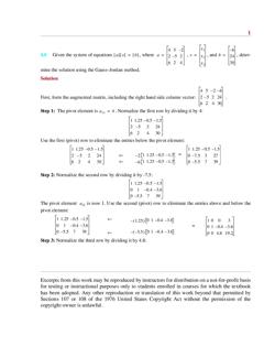
1 Excerpts from this work may be reproduced by instructors for distribution on a not-for-profit basis for testing or instructional purposes only to students enrolled in courses for which the textbook has been adopted. Any other reproduction or translation of this work beyond that permitted by 4.8 Given the system of equations , where , , and , deter- mine the solution using the Gauss–Jordan method. Solution First, form the augmented matrix, including the right hand side column vector: . Step 1: The pivot element is . Normalize the first row by dividing it by 4: Use the first (pivot) row
Numerical Methods For Engineers And Scientists: An Introduction With Applications Using Matlab 3 Chapter 4
1 Excerpts from this work may be reproduced by instructors for distribution on a not-for-profit basis for testing or instructional purposes only to students enrolled in courses for which the textbook has been adopted. Any other reproduction or translation of this work beyond that permitted by 4.43 Traffic congestion is encountered at the intersections shown in the figure. All the streets are one-way and in the directions shown. In order for effective movement of traffic, it is necessary that for every car that arrives at a given corner, another car must leave so that the number of cars arriving per unit
Numerical Methods For Engineers And Scientists: An Introduction With Applications Using Matlab 3 Chapter 4
1 Excerpts from this work may be reproduced by instructors for distribution on a not-for-profit basis for testing or instructional purposes only to students enrolled in courses for which the textbook has been adopted. Any other reproduction or translation of this work beyond that permitted by 4.15 Carry out the first three iterations of the solution of the following system of equations using the Gauss–Seidel iterative method. For the first guess of the solution, take the value of all the unknowns to be zero. Solution The essence of the Gauss-Seidel iterative method is given by Eq. (4.51): First Iteration: Starting with
Numerical Methods For Engineers And Scientists: An Introduction With Applications Using Matlab 3 Chapter 4
1 Excerpts from this work may be reproduced by instructors for distribution on a not-for-profit basis for testing or instructional purposes only to students enrolled in courses for which the textbook has been adopted. Any other reproduction or translation of this work beyond that permitted by 4.36 The axial force in each of the 17 member pin connected truss, shown in the figure, can be calculated by solving the following system of 17 equations: , ,, , ,, ,, (a) Solve the system of equations using the user-defined function GaussJordan developed in Problem 4.22. (b) Solve the system of equations using
Numerical Methods For Engineers And Scientists: An Introduction With Applications Using Matlab 3 Chapter 4
1 Excerpts from this work may be reproduced by instructors for distribution on a not-for-profit basis for testing or instructional purposes only to students enrolled in courses for which the textbook has been adopted. Any other reproduction or translation of this work beyond that permitted by 4.40 When balancing the following chemical reaction by conserving the number of atoms of each element between reactants and products: the unknown stoichiometric coefficients a, b, c, and d are given by the solution of the follow ing system of equations: Solve for the unknown stoichiometric coefficients using (a) The user-defined function GaussJordan that was
Numerical Methods For Engineers And Scientists: An Introduction With Applications Using Matlab 3 Chapter 10
1 Excerpts from this work may be reproduced by instructors for distribution on a not-for-profit basis for testing or instructional purposes only to students enrolled in courses for which the textbook has been adopted. Any other reproduction or translation of this work beyond that permitted by 10.20 The user-defined MATLAB function Sys2ODEsRK2(ODE1,ODE2,a,b,h,yINI,zINI) (Program 10-5), that is listed in the solution of Example 10-7, solves a system of two ODEs by using the second-order Runge–Kutta method (modified Euler version). Modify the function such that the two ODEs are entered in one input argument. Similarly, the domain should be entered by using one